Researchers often include control variables to block backdoor paths.
Many interpret the resulting treatment coefficient as the
average treatment effect (ATE). However, linear regression
and generalized linear model methods do not recover ATE by default.
Instead, they recover weighted strata-specific averages (Chattopadhyay
and Zubizarreta 2024). To bridge this gap, DAGassist automates estimand
recovery by constructing weights that align estimation with a
user-specified target estimand. This vignette illustrates the workflow
using a simulated dataset.
Dataset summary statistics (click to expand)
| variable | type | Min | Q1 | Median | Mean | Q3 | Max |
|---|---|---|---|---|---|---|---|
| id | integer | 1.00 | 250.75 | 500.50 | 500.50 | 750.25 | 1000.00 |
| year | integer | 0.00 | 1.00 | 2.00 | 2.00 | 3.00 | 4.00 |
| age | numeric | 0.00 | 27.60 | 37.70 | 37.76 | 47.40 | 86.20 |
| pref | numeric | 0.00 | 1.35 | 2.03 | 2.06 | 2.74 | 4.94 |
| edu_year | numeric | 0.00 | 11.80 | 13.10 | 13.07 | 15.20 | 22.00 |
| married | integer | 0.00 | 0.00 | 1.00 | 0.56 | 1.00 | 1.00 |
| birth_control | integer | 0.00 | 0.00 | 1.00 | 0.71 | 1.00 | 1.00 |
| income | numeric | 2344.00 | 43141.75 | 87560.50 | 125387.86 | 162098.50 | 1817478.00 |
| children | numeric | 0.00 | 0.00 | 0.00 | 2.03 | 3.00 | 12.00 |
| job_stability_t | numeric | -3.00 | -0.27 | 0.55 | 0.49 | 1.29 | 3.00 |
| variable | type | top_levels |
|---|---|---|
| gender | factor | Male:2565 Female:2435 |
| immigrant | factor | No:4380 Yes:620 |
| urban | factor | Urban:3560 Rural:1440 |
| class | ordered | Working:2080 Middle:1580 Low:885 (Other):455 |
| religion | factor | Christian:2005 Unaffiliated:1725 Muslim:460 (Other):810 |
| contract | factor | Temporary:1905 Permanent:1810 Informal:1285 |
| edu_degree | factor | HS_grad:1610 Some_college:1390 BA:975 (Other):1025 |
#> Warning: Removed 1 row containing missing values or values outside the scale range
#> (`geom_dag_point()`).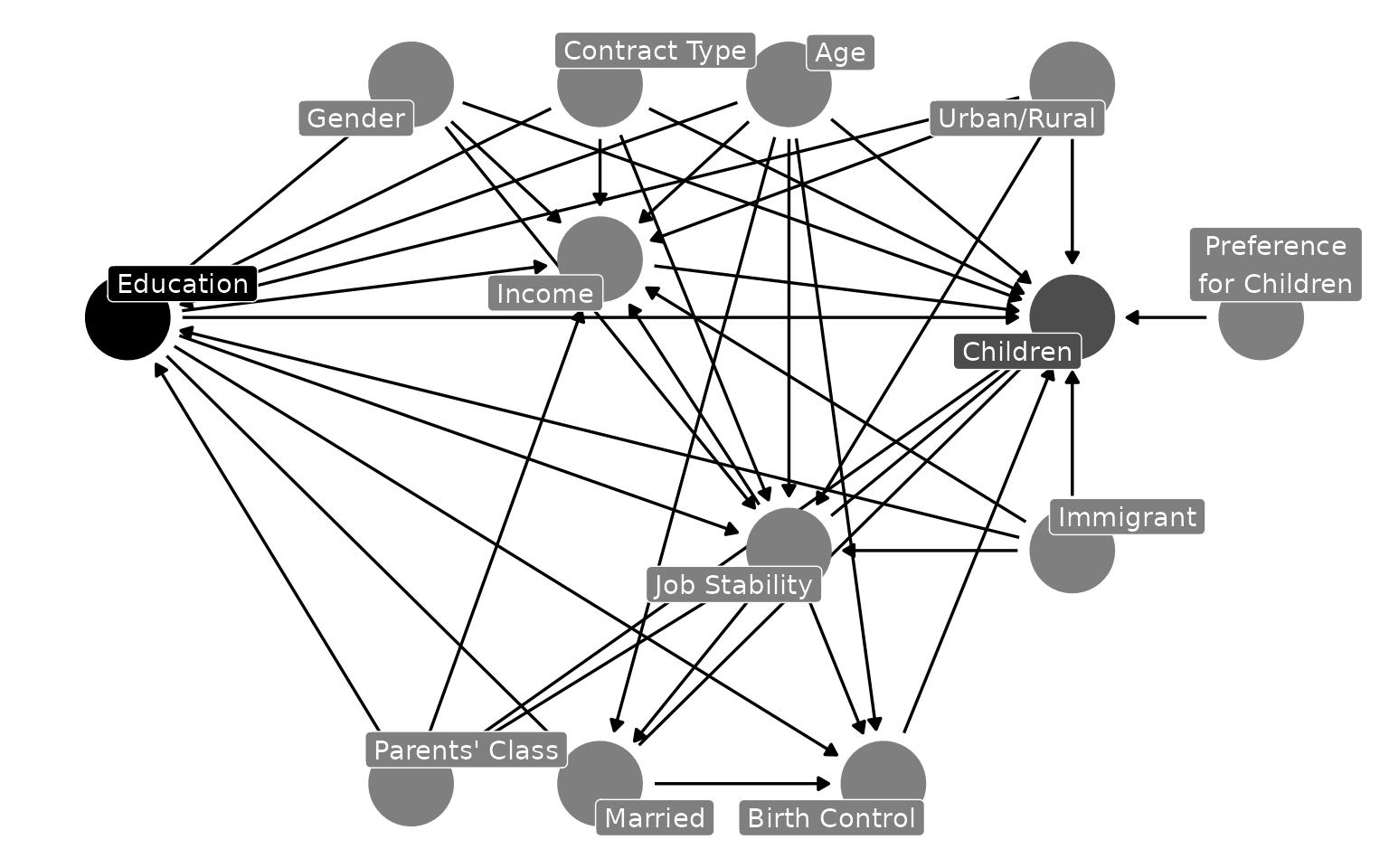
Example: The Causal Effects of Family Background and Life Course Events on Fertility Patterns
The DAG above visualizes a common social science question: how does
education affect fertility (Morgan and Winship, 17-19)? The DAG model
encodes a plausible, but not exhaustive, set of covariates. In the
report below, DAGassist classifies variables by their
causal roles, reestimates the model with DAG-consistent adjustment sets,
and recovers the ATE using weights.
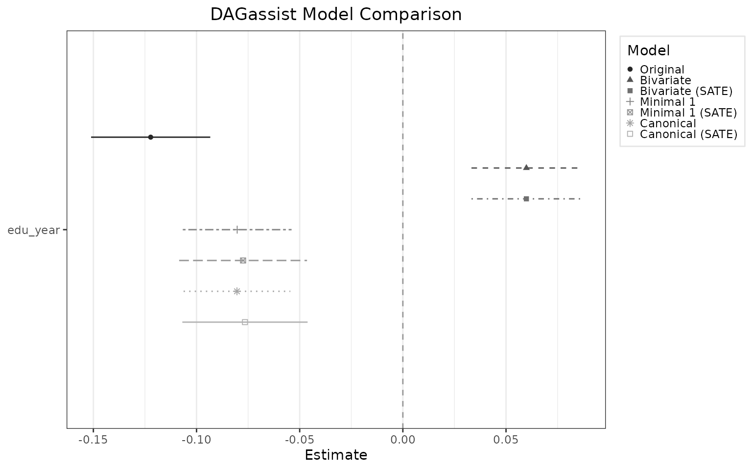
Visualizing the effect of estimand recovery
In some cases, the target estimand is the average controlled direct
effect. DAGassist supports recovering the controlled direct
effect using sequential g-estimation via integration with the
DirectEffects R package.
Using the prior example, we can use DAGassist to
estimate the effect of years of education on a person’s number of
children, except through birth control, income, and marital status.
library(DirectEffects)
#> Registered S3 method overwritten by 'DirectEffects':
#>   method    from
#>   vcov.seqg DAGassist

DAGassist(dag_model,
          formula = lm(children ~ edu_year + age + class + gender +
                         immigrant + urban + birth_control + income +
                         married + job_stability_t + contract + pref, data = dat),
          estimand = "SACDE")
#> DAGassist Report:
#>
#> Roles:
#> variable         role        Exp.  Out.  conf  med  col  dOut  dMed  dCol  dConfOn  dConfOff  NCT  NCO
#> edu_year         exposure    x
#> children         outcome           x
#> age              confounder              x
#> class            confounder              x
#> contract         confounder              x
#> gender           confounder              x
#> immigrant        confounder              x
#> urban            confounder              x
#> birth_control    mediator                      x               x
#> income           mediator                      x               x
#> job_stability_t  mediator                      x
#> married          mediator                      x               x
#> pref             nco                                                                               x
#>
#>  (!) Bad controls in your formula: {birth_control, income, married, job_stability_t}
#> Minimal controls 1: {age, class, contract, gender, immigrant, urban}
#> Canonical controls: {age, class, contract, gender, immigrant, pref, urban}
#>
#> Formulas:
#>   original:  children ~ edu_year + age + class + gender + immigrant + urban +     birth_control + income + married + job_stability_t + contract +     pref
#>
#> ACDE setup:
#>   FE-collinear dropped: (none)
#>   Formulas (sequential_g):
#>    - Original: children ~ edu_year + age + class + gender + immigrant + urban + contract + pref | 0 | birth_control + income + married + job_stability_t
#>    - Minimal 1: children ~ edu_year + age + class + contract + gender + immigrant + urban | 0 | birth_control + income + married + job_stability_t
#>    - Canonical: children ~ edu_year + age + class + contract + gender + immigrant + pref + urban | 0 | birth_control + income + married + job_stability_t
#>
#> Model comparison:
#>
#> +-------------------+-----------+-----------+-----------+------------+-----------+------------+
#> |                   | Original  | Original  | Minimal 1 | Minimal 1  | Canonical | Canonical  |
#> +===================+===========+===========+===========+============+===========+============+
#> | edu_year          | -0.122*** | -0.122*** | -0.080*** | -0.121***  | -0.080*** | -0.122***  |
#> +-------------------+-----------+-----------+-----------+------------+-----------+------------+
#> |                   | (0.015)   | (0.010)   | (0.013)   | (0.010)    | (0.013)   | (0.010)    |
#> +-------------------+-----------+-----------+-----------+------------+-----------+------------+
#> | age               | 0.070***  | 0.070***  | 0.095***  | 0.070***   | 0.096***  | 0.070***   |
#> +-------------------+-----------+-----------+-----------+------------+-----------+------------+
#> |                   | (0.004)   | (0.003)   | (0.003)   | (0.003)    | (0.003)   | (0.003)    |
#> +-------------------+-----------+-----------+-----------+------------+-----------+------------+
#> | genderMale        | 0.181*    | 0.181*    | 0.179*    | 0.171*     | 0.190*    | 0.181*     |
#> +-------------------+-----------+-----------+-----------+------------+-----------+------------+
#> |                   | (0.085)   | (0.085)   | (0.087)   | (0.086)    | (0.085)   | (0.085)    |
#> +-------------------+-----------+-----------+-----------+------------+-----------+------------+
#> | immigrantYes      | -0.246+   | -0.246*   | -0.172    | -0.175     | -0.243+   | -0.246*    |
#> +-------------------+-----------+-----------+-----------+------------+-----------+------------+
#> |                   | (0.128)   | (0.116)   | (0.131)   | (0.118)    | (0.129)   | (0.116)    |
#> +-------------------+-----------+-----------+-----------+------------+-----------+------------+
#> | urbanUrban        | 0.121     | 0.121     | 0.238*    | 0.190*     | 0.175+    | 0.121      |
#> +-------------------+-----------+-----------+-----------+------------+-----------+------------+
#> |                   | (0.094)   | (0.090)   | (0.096)   | (0.092)    | (0.094)   | (0.090)    |
#> +-------------------+-----------+-----------+-----------+------------+-----------+------------+
#> | birth_control     | 0.133     |           |           |            |           |            |
#> +-------------------+-----------+-----------+-----------+------------+-----------+------------+
#> |                   | (0.103)   |           |           |            |           |            |
#> +-------------------+-----------+-----------+-----------+------------+-----------+------------+
#> | income            | 0.000     |           |           |            |           |            |
#> +-------------------+-----------+-----------+-----------+------------+-----------+------------+
#> |                   | (0.000)   |           |           |            |           |            |
#> +-------------------+-----------+-----------+-----------+------------+-----------+------------+
#> | married           | 0.703***  |           |           |            |           |            |
#> +-------------------+-----------+-----------+-----------+------------+-----------+------------+
#> |                   | (0.122)   |           |           |            |           |            |
#> +-------------------+-----------+-----------+-----------+------------+-----------+------------+
#> | job_stability_t   | 0.285***  |           |           |            |           |            |
#> +-------------------+-----------+-----------+-----------+------------+-----------+------------+
#> |                   | (0.047)   |           |           |            |           |            |
#> +-------------------+-----------+-----------+-----------+------------+-----------+------------+
#> | contractTemporary | 0.710***  | 0.710***  | 0.772***  | 0.685***   | 0.804***  | 0.710***   |
#> +-------------------+-----------+-----------+-----------+------------+-----------+------------+
#> |                   | (0.110)   | (0.102)   | (0.112)   | (0.103)    | (0.110)   | (0.102)    |
#> +-------------------+-----------+-----------+-----------+------------+-----------+------------+
#> | contractPermanent | 0.893***  | 0.893***  | 1.116***  | 0.932***   | 1.093***  | 0.893***   |
#> +-------------------+-----------+-----------+-----------+------------+-----------+------------+
#> |                   | (0.114)   | (0.102)   | (0.113)   | (0.104)    | (0.111)   | (0.102)    |
#> +-------------------+-----------+-----------+-----------+------------+-----------+------------+
#> | pref              | 0.581***  | 0.581***  |           |            | 0.578***  | 0.581***   |
#> +-------------------+-----------+-----------+-----------+------------+-----------+------------+
#> |                   | (0.042)   | (0.046)   |           |            | (0.042)   | (0.046)    |
#> +-------------------+-----------+-----------+-----------+------------+-----------+------------+
#> | Num.Obs.          | 5000      | 5000      | 5000      | 5000       | 5000      | 5000       |
#> +-------------------+-----------+-----------+-----------+------------+-----------+------------+
#> | R2                | 0.227     |           | 0.183     |            | 0.213     |            |
#> +===================+===========+===========+===========+============+===========+============+
#> | + p < 0.1, * p < 0.05, ** p < 0.01, *** p < 0.001                                           |
#> +===================+===========+===========+===========+============+===========+============+
#>
#> Roles legend: Exp. = exposure; Out. = outcome; CON = confounder; MED = mediator; COL = collider; dOut = descendant of outcome; dMed  = descendant of mediator; dCol = descendant of collider; dConfOn = descendant of a confounder on a back-door path; dConfOff = descendant of a confounder off a back-door path; NCT = neutral control on treatment; NCO = neutral control on outcome