Getting Started with Report Creation

Introduction

This vignette explains how to make publication-grade DAGassist reports in LaTeX, Word, Excel, and plaintext. Since this package’s primary utility is as a robustness check for observational studies, most of its functionality revolves around creating reports.

Install and load `DAGassist`

# install development release from github
install.packages("pak")
pak::pak("grahamgoff/DAGassist")

# or, install stable release from CRAN
install.packages("DAGassist")

#load DAGassist
library(DAGassist)

Setup

In addition to loading DAGassist, we will load the following baseline packages:

modelsummary to build the model comparison table for LaTeX, Word, Excel, and plaintext.
- LaTeX uses broom as a fallback for report generation
knitr to build intermediate .md for Word and plaintext report generation.
rmarkdown to convert .md files to .docx files for Word report generation.
writexl to export Excel files.

Essentially, to export:

LaTeX only needs modelsummary
Excel needs modelsummary and writexl
plaintext needs modelsummary and knitr
Word needs modelsummary, knitr, and rmarkdown

#load libraries to help export
library(modelsummary)
library(writexl)
library(knitr)
library(rmarkdown)

Example DAG

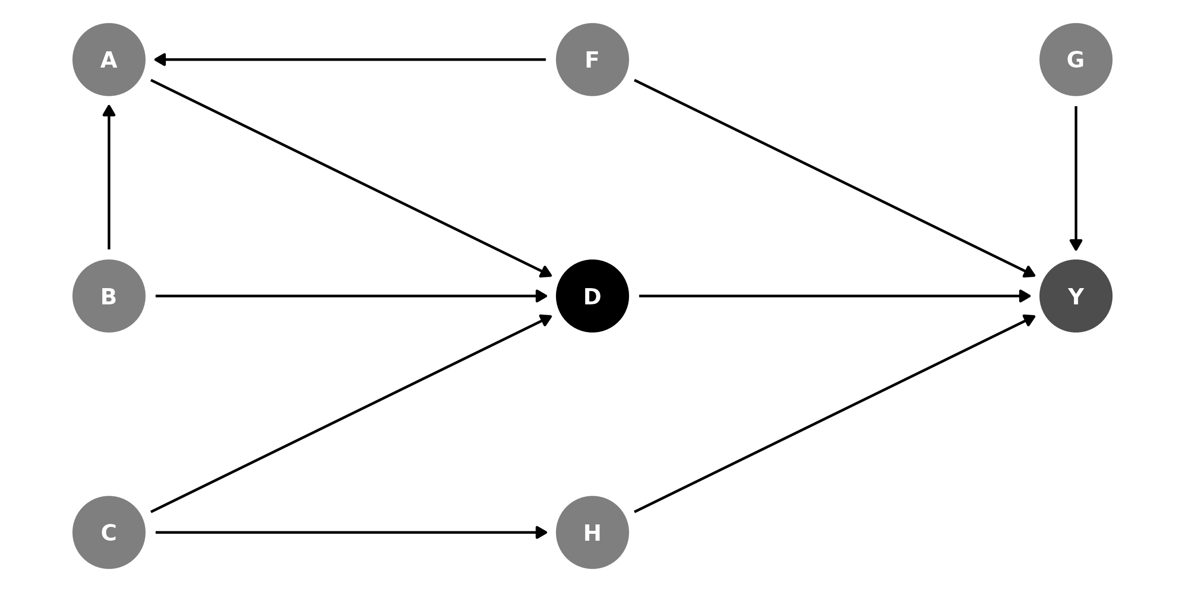
The data, which simulates the DAG relationships:

head(df)
#>            Y          D          H          A           G          F
#> 1 -4.3598990 -1.7293707 -1.2908129 -0.3906503 -0.15030748 -0.5116037
#> 2  1.6129050  1.0748492  0.2956294  0.6771872 -0.32775713  0.2369379
#> 3  1.5096451  1.0922811 -1.1613337  1.1254048 -1.44816529 -0.5415892
#> 4  1.1554071 -0.5867292  1.3752785 -0.5173670 -0.69728458  1.2192276
#> 5  0.2920729 -2.0225129 -1.1232830 -1.8569842  2.59849023  0.1741359
#> 6  3.1428430  3.0900447  1.1675898  2.6936976 -0.03741501 -0.6152683
#>             C           B
#> 1 -0.99579872 -0.56047565
#> 2 -1.03995504 -0.23017749
#> 3 -0.01798024  1.55870831
#> 4 -0.13217513  0.07050839
#> 5 -2.54934277  0.12928774
#> 6  1.04057346  1.71506499

Creating a report

Suppose you wrote an article uses model original as its main finding, and you want to ensure that your specification captures the total effect of D on Y, without mediator or collider bias.

original <- lm(Y ~ D + G + H + F + A + B + C, data = df)

DAGassist can generate a report assessing the causal roles of the variables in original.

DAGassist(dag = dag_model, #specify a dagitty or ggdag object
          formula = lm(Y ~ D + G + H + F + A + B + C, data = df), #provide your formula
          type = "text", #output type
          out = out_txt) #a temporary directory, for the purpose of this vignette

cat(readLines(out_txt), sep = "\n") # show the output

DAGassist Report:

Roles

Variable	Role	Exp.	Out.	`CON`	dConfOn	`NCO`
A	confounder			x	x
B	confounder			x
C	confounder			x
D	exposure	x
F	confounder			x
G	nco					x
H	nco				x	x
Y	outcome		x

Models

Term	Original	Minimal 1	Minimal 2	Minimal 3	Minimal 4	Canonical
D	1.034***	0.977***	0.969***	1.038***	1.024***	1.034***
	(0.032)	(0.020)	(0.023)	(0.036)	(0.041)	(0.032)
G	0.397***					0.397***
	(0.032)					(0.032)
H	0.486***	0.522***		0.495***		0.486***
	(0.032)	(0.028)		(0.031)		(0.032)
F	0.618***	0.606***	0.593***			0.618***
	(0.037)	(0.036)	(0.040)			(0.037)
A	-0.111**			0.158***	0.169***	-0.111**
	(0.043)			(0.047)	(0.051)	(0.043)
B	-0.008			-0.161***	-0.162***	-0.008
	(0.039)			(0.045)	(0.049)	(0.039)
C	0.037		0.420***		0.391***	0.037
	(0.042)		(0.040)		(0.045)	(0.042)
Num.Obs.	1000	1000	1000	1000	1000	1000
R2	0.836	0.809	0.769	0.762	0.724	0.836

Notes

Roles legend: X (exposure); Y (outcome); CON (confounder); MED (mediator); COL (collider); dOut (proper descendant of Y); dMed (proper descendant of any mediator); dCol (proper descendant of any collider); dConfOn (descendant of a confounder on a back-door path); dConfOff (descendant of a confounder off a back-door path); NCT (neutral control on treatment); NCO (neutral control on outcome).
p-value legend: + < 0.1, * < 0.05, ** < 0.01, *** < 0.001.
Controls (minimal): {F, H}.
Controls (canonical): {A, B, C, F, G, H}.

Creating sub-reports (roles-only or models-only)

Sometimes you only need one part of the report. Use the show argument to generate just the roles grid or just the model comparison:

show = "roles" – produce only the DAG-based roles table.
No model is fitted, and no formula or data is required. This is ideal when your regression engine isn’t supported or you simply want to audit variable roles.
show = "models" – produce only the model comparison (Original / Minimal / Canonical).
Requires a model specification (either a formula or a single engine call); no roles table is printed.

Examples

DAGassist(dag = dag_model,
          show = "roles")
#> DAGassist Report: 
#> 
#> Roles:
#> variable  role        Exp.  Out.  conf  med  col  dOut  dMed  dCol  dConfOn  dConfOff  NCT  NCO
#> D         exposure    x                                                                        
#> Y         outcome           x                                                                  
#> A         confounder              x                                 x                          
#> B         confounder              x                                                            
#> C         confounder              x                                                            
#> F         confounder              x                                                            
#> G         nco                                                                               x  
#> H         nco                                                       x                       x  
#> 
#> Roles legend: Exp. = exposure; Out. = outcome; CON = confounder; MED = mediator; COL = collider; dOut = descendant of outcome; dMed  = descendant of mediator; dCol = descendant of collider; dConfOn = descendant of a confounder on a back-door path; dConfOff = descendant of a confounder off a back-door path; NCT = neutral control on treatment; NCO = neutral control on outcome

Making a dot‑whisker plot of the key coefficient

# Returns a ggplot object (prints if out = NULL; saves if out is a file path)
DAGassist(dag = dag_model,
          formula = lm(Y ~ D + G + H + F + A + B + C, data = df),
          type = "dotwhisker")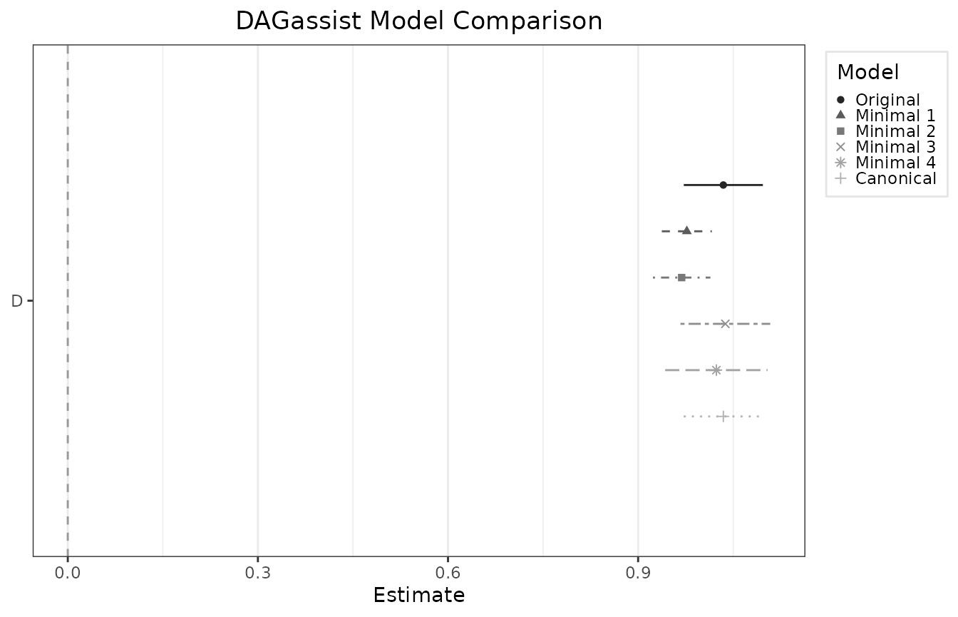

Using special canonical sets

By default, DAGassist() reports the canonical adjustment set, which only excludes non-admissible adjustments (colliders, mediators, and their descendants). Sometimes, users may want to see the canonical set minus certain classes of “neutral” controls, per Hunermund, Louw and Ronkko (2025). The exclude = argument enables selective exclusion of neutral controls.

exclude = "nct" drops neutral controls on the treatment
exclude = "nco" drops neutral controls on the outcome

DAGassist(dag = dag_model,
          formula = lm(Y ~ D + G + H + F + A + B + C, data = df),
          exclude = c("nct", "nco"),
          show = "models",
          type = "text")

DAGassist Report:

Models

Term	Original	Minimal 1	Minimal 2	Minimal 3	Minimal 4	Canonical	Canon. (-NCT)	Canon. (-NCO)
D	1.034***	0.977***	0.969***	1.038***	1.024***	1.034***	1.034***	1.019***
	(0.032)	(0.020)	(0.023)	(0.036)	(0.041)	(0.032)	(0.032)	(0.038)
G	0.397***					0.397***	0.397***
	(0.032)					(0.032)	(0.032)
H	0.486***	0.522***		0.495***		0.486***	0.486***
	(0.032)	(0.028)		(0.031)		(0.032)	(0.032)
F	0.618***	0.606***	0.593***			0.618***	0.618***	0.618***
	(0.037)	(0.036)	(0.040)			(0.037)	(0.037)	(0.044)
A	-0.111**			0.158***	0.169***	-0.111**	-0.111**	-0.088+
	(0.043)			(0.047)	(0.051)	(0.043)	(0.043)	(0.050)
B	-0.008			-0.161***	-0.162***	-0.008	-0.008	-0.013
	(0.039)			(0.045)	(0.049)	(0.039)	(0.039)	(0.046)
C	0.037		0.420***		0.391***	0.037	0.037	0.403***
	(0.042)		(0.040)		(0.045)	(0.042)	(0.042)	(0.041)
Num.Obs.	1000	1000	1000	1000	1000	1000	1000	1000
R2	0.836	0.809	0.769	0.762	0.724	0.836	0.836	0.770

Notes

p-value legend: + < 0.1, * < 0.05, ** < 0.01, *** < 0.001.
Controls (minimal): {F, H}.
Controls (canonical): {A, B, C, F, G, H}.

Introduction

Install and load DAGassist

Setup

Example DAG

Creating a report

DAGassist Report:

Roles

Models

Notes

Creating sub-reports (roles-only or models-only)

Examples

Making a dot‑whisker plot of the key coefficient

Using special canonical sets

DAGassist Report:

Models

Notes

Install and load `DAGassist`